Logistic Regression is a classification algorithm and not a regression algorithm. It is used to estimate discrete values (like 0 or 1, True or False, Yes or No) based on a given set of independent variables.
Logistic Regression produces results in a binary format that is used to predict the outcome of a categorical dependent variable. So the outcome should be discrete/categorical.
Dataset
We will be using a simple dataset to implement this algorithm. This dataset contains User ID, Gender, Age, Estimated Salary and Purchased column. Purchased column has data as 0 and 1 where 1 denotes that car is purchased.
Download the dataset here.
So let’s begin here…
import pandas as pd
import numpy as np
import matplotlib.pyplot as plt
import seaborn as sns

from sklearn.linear_model import LogisticRegression
from sklearn.model_selection import train_test_split
from sklearn.preprocessing import StandardScaler
from sklearn.metrics import classification_report
from sklearn.metrics import confusion_matrix
from sklearn.metrics import accuracy_score
Load Data
data = pd.read_csv("suv.csv")
data.head(10)
| User ID | Gender | Age | EstimatedSalary | Purchased | |
|---|---|---|---|---|---|
| 0 | 15624510 | Male | 19 | 19000 | 0 |
| 1 | 15810944 | Male | 35 | 20000 | 0 |
| 2 | 15668575 | Female | 26 | 43000 | 0 |
| 3 | 15603246 | Female | 27 | 57000 | 0 |
| 4 | 15804002 | Male | 19 | 76000 | 0 |
| 5 | 15728773 | Male | 27 | 58000 | 0 |
| 6 | 15598044 | Female | 27 | 84000 | 0 |
| 7 | 15694829 | Female | 32 | 150000 | 1 |
| 8 | 15600575 | Male | 25 | 33000 | 0 |
| 9 | 15727311 | Female | 35 | 65000 | 0 |
print("Number of customers: ", len(data))
Number of customers: 400
Analyzing Data
data.info()
<class 'pandas.core.frame.DataFrame'>
RangeIndex: 400 entries, 0 to 399
Data columns (total 5 columns):
User ID            400 non-null int64
Gender             400 non-null object
Age                400 non-null int64
EstimatedSalary    400 non-null int64
Purchased          400 non-null int64
dtypes: int64(4), object(1)
memory usage: 15.7+ KB
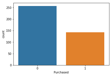
Customers who purchased the SUV
sns.countplot(x='Purchased', data = data)
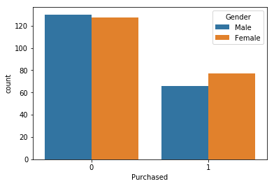
Customers who purchased the SUV based on Gender
sns.countplot(x='Purchased', hue = 'Gender', data = data)
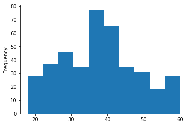
Graph for age of customers
data['Age'].plot.hist()
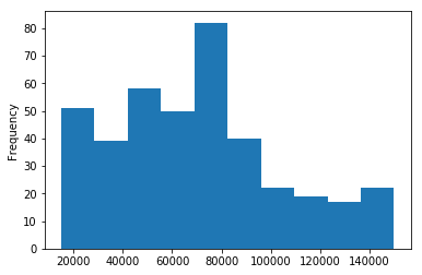
Graph for Estimated Salary of Customers
data['EstimatedSalary'].plot.hist()
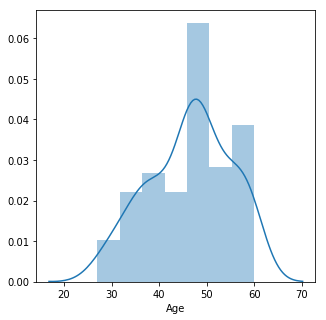
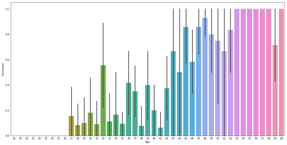
Customers who purchased the SUV based on Age
plt.figure(figsize = (5,5))
sns.distplot(data[data['Purchased']==1]['Age'])
plt.figure(figsize = (20,10))
sns.barplot(x=data['Age'],y=data['Purchased'])
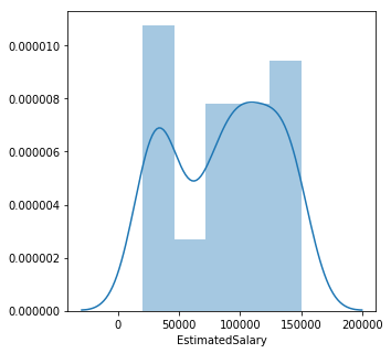
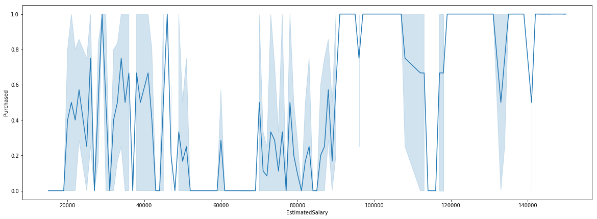
Customers who purchased the SUV based on Estimated Salary
plt.figure(figsize = (5,5))
sns.distplot(data[data['Purchased']==1]['EstimatedSalary'])
plt.figure(figsize = (20,7))
sns.lineplot(x=data['EstimatedSalary'],y=data['Purchased'])
Preprocessing
Gender = pd.get_dummies(data['Gender'], drop_first = True)
Gender.head(5)
| Male | |
|---|---|
| 0 | 1 |
| 1 | 1 |
| 2 | 0 |
| 3 | 0 |
| 4 | 1 |
data = pd.concat([data, Gender], axis = 1)
Dropping User ID and Gender column
data.drop(['User ID', 'Gender'], axis = 1, inplace = True)
data.head()
| Age | EstimatedSalary | Purchased | Male | |
|---|---|---|---|---|
| 0 | 19 | 19000 | 0 | 1 |
| 1 | 35 | 20000 | 0 | 1 |
| 2 | 26 | 43000 | 0 | 0 |
| 3 | 27 | 57000 | 0 | 0 |
| 4 | 19 | 76000 | 0 | 1 |
Dependent and Independent variables
X = data.drop('Purchased', axis = 1)
y = data['Purchased']
Train and Test data
X_train, X_test, y_train, y_test = train_test_split(X, y, test_size = 0.2, random_state = 1)
sc = StandardScaler()
X_train = sc.fit_transform(X_train)
X_test = sc.transform(X_test)
Define Model
model = LogisticRegression(solver = 'liblinear')
Fit Model
model.fit(X_train,y_train)
LogisticRegression(C=1.0, class_weight=None, dual=False, fit_intercept=True,
          intercept_scaling=1, max_iter=100, multi_class='warn',
          n_jobs=None, penalty='l2', random_state=None, solver='liblinear',
          tol=0.0001, verbose=0, warm_start=False)
Predictions
predictions = model.predict(X_test)
Classification Report
print(classification_report(y_test, predictions))
              precision    recall  f1-score   support

           0       0.87      0.83      0.85        48
           1       0.76      0.81      0.79        32

   micro avg       0.82      0.82      0.82        80
   macro avg       0.82      0.82      0.82        80
weighted avg       0.83      0.82      0.83        80
Confusion Matrix
It is a 2x2 matrix that has 4 outcomes. This tells how accurate the values are.
print("Confusion Matrix: \n",confusion_matrix(y_test, predictions))
Confusion Matrix:
 [[40  8]
 [ 6 26]]
Accuracy
print("Accuracy: ",accuracy_score(y_test, predictions))
Accuracy: 0.825