Context
This dataset is originally from the National Institute of Diabetes and Digestive and Kidney Diseases. The objective of the dataset is to diagnostically predict whether or not a patient has diabetes, based on certain diagnostic measurements included in the dataset. Several constraints were placed on the selection of these instances from a larger database. In particular, all patients here are females at least 21 years old of Pima Indian heritage.
Content
The datasets consists of several medical predictor variables and one target variable, Outcome. Predictor variables includes the number of pregnancies the patient has had, their BMI, insulin level, age, and so on.
Acknowledgements
Smith, J.W., Everhart, J.E., Dickson, W.C., Knowler, W.C., & Johannes, R.S. (1988). Using the ADAP learning algorithm to forecast the onset of diabetes mellitus. In Proceedings of the Symposium on Computer Applications and Medical Care (pp. 261–265). IEEE Computer Society Press.
Inspiration
Can you build a machine learning model to accurately predict whether or not the patients in the dataset have diabetes or not?
So let’s begin here
import numpy as np
import pandas as pd
import matplotlib.pyplot as plt

%matplotlib inline
Load Data
data = pd.read_csv("pima-csv.csv")
data.shape
(768, 9)
data.head(5)
| Pregnancies | Glucose | BloodPressure | SkinThickness | Insulin | BMI | DiabetesPedigreeFunction | Age | Outcome | |
|---|---|---|---|---|---|---|---|---|---|
| 0 | 6 | 148 | 72 | 35 | 0 | 33.6 | 0.627 | 50 | 1 |
| 1 | 1 | 85 | 66 | 29 | 0 | 26.6 | 0.351 | 31 | 0 |
| 2 | 8 | 183 | 64 | 0 | 0 | 23.3 | 0.672 | 32 | 1 |
| 3 | 1 | 89 | 66 | 23 | 94 | 28.1 | 0.167 | 21 | 0 |
| 4 | 0 | 137 | 40 | 35 | 168 | 43.1 | 2.288 | 33 | 1 |
data.info()
<class 'pandas.core.frame.DataFrame'>
RangeIndex: 768 entries, 0 to 767
Data columns (total 9 columns):
Pregnancies                 768 non-null int64
Glucose                     768 non-null int64
BloodPressure               768 non-null int64
SkinThickness               768 non-null int64
Insulin                     768 non-null int64
BMI                         768 non-null float64
DiabetesPedigreeFunction    768 non-null float64
Age                         768 non-null int64
Outcome                     768 non-null int64
dtypes: float64(2), int64(7)
memory usage: 54.1 KB
data.isnull().sum()
Pregnancies                 0
Glucose                     0
BloodPressure               0
SkinThickness               0
Insulin                     0
BMI                         0
DiabetesPedigreeFunction    0
Age                         0
Outcome                     0
dtype: int64
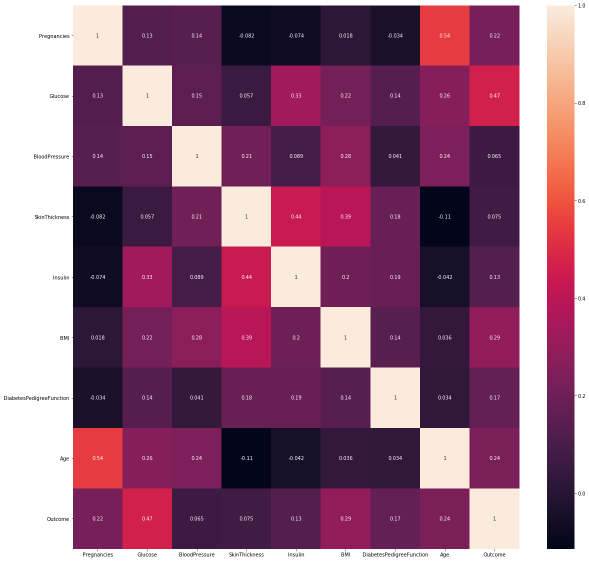
Correlation
import seaborn as sns
corr_ds = data.corr()
top_corr = corr_ds.index
plt.figure(figsize=(20,20))
g = sns.heatmap(data[top_corr].corr(), annot = True)
data.corr()
| Pregnancies | Glucose | BloodPressure | SkinThickness | Insulin | BMI | DiabetesPedigreeFunction | Age | Outcome | |
|---|---|---|---|---|---|---|---|---|---|
| Pregnancies | 1.000000 | 0.129459 | 0.141282 | -0.081672 | -0.073535 | 0.017683 | -0.033523 | 0.544341 | 0.221898 |
| Glucose | 0.129459 | 1.000000 | 0.152590 | 0.057328 | 0.331357 | 0.221071 | 0.137337 | 0.263514 | 0.466581 |
| BloodPressure | 0.141282 | 0.152590 | 1.000000 | 0.207371 | 0.088933 | 0.281805 | 0.041265 | 0.239528 | 0.065068 |
| SkinThickness | -0.081672 | 0.057328 | 0.207371 | 1.000000 | 0.436783 | 0.392573 | 0.183928 | -0.113970 | 0.074752 |
| Insulin | -0.073535 | 0.331357 | 0.088933 | 0.436783 | 1.000000 | 0.197859 | 0.185071 | -0.042163 | 0.130548 |
| BMI | 0.017683 | 0.221071 | 0.281805 | 0.392573 | 0.197859 | 1.000000 | 0.140647 | 0.036242 | 0.292695 |
| DiabetesPedigreeFunction | -0.033523 | 0.137337 | 0.041265 | 0.183928 | 0.185071 | 0.140647 | 1.000000 | 0.033561 | 0.173844 |
| Age | 0.544341 | 0.263514 | 0.239528 | -0.113970 | -0.042163 | 0.036242 | 0.033561 | 1.000000 | 0.238356 |
| Outcome | 0.221898 | 0.466581 | 0.065068 | 0.074752 | 0.130548 | 0.292695 | 0.173844 | 0.238356 | 1.000000 |
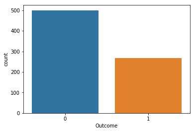
sns.countplot(data['Outcome'])
Train Data
X = data.drop(['Outcome'], axis = 1)
y = data['Outcome']
from sklearn.model_selection import train_test_split
X_train, X_test, y_train, y_test = train_test_split(X, y, test_size = 0.2, random_state = 10)
from sklearn.metrics import confusion_matrix, accuracy_score
XGBoost
import xgboost
from sklearn.model_selection import RandomizedSearchCV

xgb_model = xgboost.XGBClassifier()
param = {
    'learning_rate':[0.05,0.1,0.15,0.2,0.25,0.3],
    'max_depth':[3,4,5,6,8,10,12],
    'min_child_weight':[1,3,5,7],
    'gamma':[0.0,0.1,0.2,0.3,0.4],
    'colsample_bytree':[0.3,0.4,0.5,0.7]
}
random_search = RandomizedSearchCV(xgb_model, param_distributions = param, n_iter = 5,
                                     scoring = 'roc_auc', n_jobs = -1, cv = 5, verbose = 3)
random_search.fit(X_train,y_train)
Fitting 5 folds for each of 5 candidates, totalling 25 fits

[Parallel(n_jobs=-1)]: Using backend LokyBackend with 4 concurrent workers.
[Parallel(n_jobs=-1)]: Done  25 out of  25 | elapsed:   13.0s finished

RandomizedSearchCV(cv=5, error_score='raise-deprecating',
          estimator=XGBClassifier(base_score=None, booster=None, colsample_bylevel=None,
       colsample_bynode=None, colsample_bytree=None, gamma=None,
       gpu_id=None, importance_type='gain', interaction_constraints=None,
       learning_rate=None, max_delta_step=None, max_depth=None,
       min_child_w..._pos_weight=None, subsample=None,
       tree_method=None, validate_parameters=None, verbosity=None),
          fit_params=None, iid='warn', n_iter=5, n_jobs=-1,
          param_distributions={'learning_rate': [0.05, 0.1, 0.15, 0.2, 0.25, 0.3], 'max_depth': [3, 4, 5, 6, 8, 10, 12], 'min_child_weight': [1, 3, 5, 7], 'gamma': [0.0, 0.1, 0.2, 0.3, 0.4], 'colsample_bytree': [0.3, 0.4, 0.5, 0.7]},
          pre_dispatch='2*n_jobs', random_state=None, refit=True,
          return_train_score='warn', scoring='roc_auc', verbose=3)
random_search.best_estimator_
XGBClassifier(base_score=0.5, booster='gbtree', colsample_bylevel=1,
       colsample_bynode=1, colsample_bytree=0.3, gamma=0.1, gpu_id=-1,
       importance_type='gain', interaction_constraints='',
       learning_rate=0.05, max_delta_step=0, max_depth=12,
       min_child_weight=3, missing=nan, monotone_constraints='()',
       n_estimators=100, n_jobs=0, num_parallel_tree=1,
       objective='binary:logistic', random_state=0, reg_alpha=0,
       reg_lambda=1, scale_pos_weight=1, subsample=1, tree_method='exact',
       validate_parameters=1, verbosity=None)
xgb_model = xgboost.XGBClassifier(base_score=0.5, booster='gbtree', colsample_bylevel=1,
       colsample_bynode=1, colsample_bytree=0.3, gamma=0.1, gpu_id=-1,
       importance_type='gain', interaction_constraints='',
       learning_rate=0.05, max_delta_step=0, max_depth=12,
       min_child_weight=3, monotone_constraints='()',
       n_estimators=100, n_jobs=0, num_parallel_tree=1,
       objective='binary:logistic', random_state=0, reg_alpha=0,
       reg_lambda=1, scale_pos_weight=1, subsample=1, tree_method='exact',
       validate_parameters=1, verbosity=None)
xgb_model.fit(X_train,y_train)
XGBClassifier(base_score=0.5, booster='gbtree', colsample_bylevel=1,
       colsample_bynode=1, colsample_bytree=0.3, gamma=0.1, gpu_id=-1,
       importance_type='gain', interaction_constraints='',
       learning_rate=0.05, max_delta_step=0, max_depth=12,
       min_child_weight=3, missing=nan, monotone_constraints='()',
       n_estimators=100, n_jobs=0, num_parallel_tree=1,
       objective='binary:logistic', random_state=0, reg_alpha=0,
       reg_lambda=1, scale_pos_weight=1, subsample=1, tree_method='exact',
       validate_parameters=1, verbosity=None)
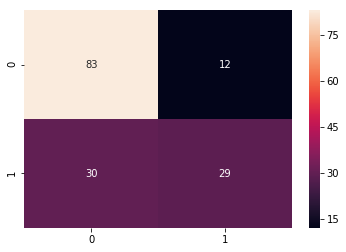
Predictions
pred_xgb = xgb_model.predict(X_test)

acc_xgb = accuracy_score(y_test,pred_xgb)
print("Accuracy XGB:", acc_xgb)
Accuracy XGB: 0.7272727272727273
cm_xgb = confusion_matrix(y_test,pred_xgb)
sns.heatmap(cm_xgb, annot=True)
Confusion Matrix
Support Vector Classifier
from sklearn.svm import SVC
from sklearn.pipeline import make_pipeline
from sklearn.preprocessing import StandardScaler

svc_model = make_pipeline(StandardScaler(), SVC(gamma='auto'))

svc_model.fit(X_train, y_train)
Pipeline(memory=None,
     steps=[('standardscaler', StandardScaler(copy=True, with_mean=True, with_std=True)), ('svc', SVC(C=1.0, cache_size=200, class_weight=None, coef0=0.0,
  decision_function_shape='ovr', degree=3, gamma='auto', kernel='rbf',
  max_iter=-1, probability=False, random_state=None, shrinking=True,
  tol=0.001, verbose=False))])
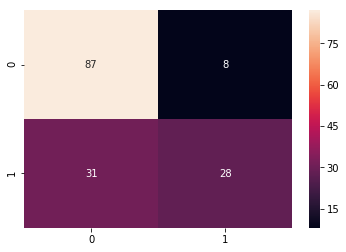
Predictions
pred_svc = svc_model.predict(X_test)

acc_svc = accuracy_score(y_test,pred_svc)
print("Accuracy SVC:", acc_svc)
Accuracy SVC: 0.7467532467532467
cm_svc = confusion_matrix(y_test,pred_svc)
sns.heatmap(cm_svc, annot=True)
Confusion Matrix
Accuracy for other algorithms
Accuracy : 0.7142857142857143 (Random Forest)
Accuracy : 0.727272727272727 (XGBoost)
Accuracy : 0.7337662337662337 (Logistic Regression)
Accuracy : 0.7467532467532467 (Support Vector Classifier)
Accuracy : 0.7012987012987013 (Decision Tree)
Accuracy : 0.7142857142857143 (Naive Bayes)
Accuracy : 0.512987012987013 (Stochastic Gradient Descent)
Accuracy : 0.7077922077922078 (K Nearest Neighbor)