Linear Regression is a statistical model that attempts to show the relationship between two variables using a Linear Equation.
What is Regression?
Regression analysis is a form of predictive modeling technique that investigates the relationship between a dependent and independent variable.
So, in linear regression, we establish a relationship between the independent and dependent variables by fitting the best line. This best fit line is known as the regression line and represented by a linear equation.
y = mx + C
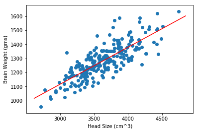
Graphical Representation

The dots in blue are the data points and the line in red is the regression line.
Dataset
We will be using a simple dataset to implement this algorithm. This dataset contains Head Size (cm^3) and Brain Weight (grams) columns where Head Size is an independent variable.
Download the dataset here.
Let’s implement this mathematically first.
So let’s begin here…
import numpy as np
import pandas as pd
import matplotlib.pyplot as plt
Load Data
data = pd.read_csv('headbrain.csv')
X=data['Head Size(cm^3)'].values
Y=data['Brain Weight(grams)'].values
print(data.head())
   Gender  Age Range  Head Size(cm^3)  Brain Weight(grams)
0       1          1             4512                 1530
1       1          1             3738                 1297
2       1          1             4261                 1335
3       1          1             3777                 1282
4       1          1             4177                 1590
Calculating mean of Head Size(X) and Brain Weight(Y)
mean_x = np.mean(X)
mean_y = np.mean(Y)

# Total number of Values
n = len(X)
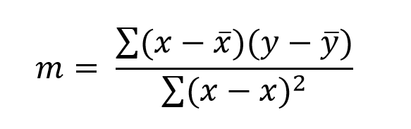
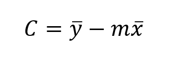
Calculating m and C
numer = 0
denom = 0

for i in range (n):
    numer += (X[i]-mean_x) * (Y[i]-mean_y)
    denom += (X[i]-mean_x)**2
m = numer/denom
c = mean_y - m * mean_x
Plotting Graph
max_x = np.max(X) + 100
min_x = np.min(X) - 100
# Calculating linvalues of x and y
x = np.linspace(min_x,max_x,1000)
y = m*x + c

plt.plot(x,y,color = 'red' ,label='Regression Line')
plt.scatter(X,Y,label='Scatter Plot')
plt.xlabel('Head Size (cm^3)')
plt.ylabel('Brain Weight (gms)')
plt.show()
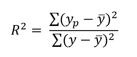
R-Squared Method
R-Squared value is a statistical measure of how close the data points are to the fitted regression line. This is also known as Coefficient of determination or Coefficient of multiple determination.
snumer = 0
sdenom = 0
for i in range(n):
    yp = m*X[i] + c
    snumer += (yp-mean_y)**2
    sdenom += (Y[i] - mean_y)**2

r2 = (snumer/sdenom)
print('R^2 value: ',r2)
R^2 value: 0.6393117199570001
Let’s implement the same using Sklearn
from sklearn.linear_model import LinearRegression
from sklearn.metrics import mean_squared_error

X = X.reshape((n,1))
Define Model
model = LinearRegression()
Fit Model
model = model.fit(X,Y)
Calculating R^2
r2 = model.score(X,Y)
print('R^2 value: ',r2)
R^2 value: 0.639311719957
Predictions
Y_pred = model.predict(X)
Model Deployment
The model for above algorithm is deployed on Heroku. You can check here.